Visualizing Data

The imfusion package enables to launch a detached window that displays Data (e.g., a SharedImageSet) or a list of Data.

As an example, a list of Data is obtained when loading an image from disk using load(). Afterwards, the image can simply be displayed by calling show() and passing it the list of data:

>>> data_list = imfusion.load(data_path) 
>>> imfusion.show(data_list, title="s0004")
<imfusion.VisualizerHandle object at...>

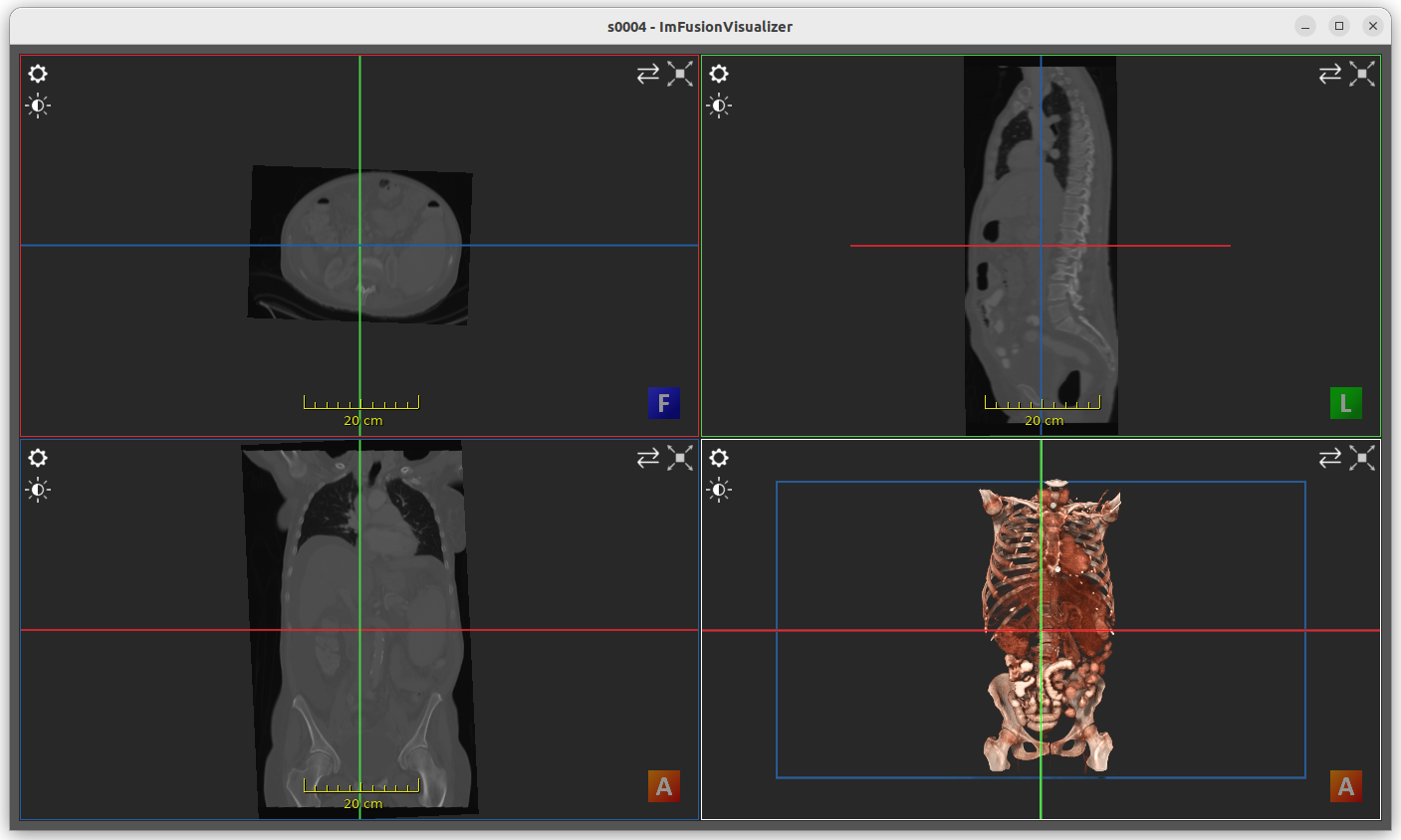
An ImFusionVisualizer instance

Furthermore, show() returns a VisualizerHandle instance that allows to inspect some basic information or to close the visualizer when needed:

>>> visualizer_handle = imfusion.show(data_list, title="s0004")
>>> print(visualizer_handle.title())
s0004
>>> ...  
>>> visualizer_handle.close()

All open visualizers can be closed simultaneously with close_viewers(). To see which visualizers are currently open, use list_viewers(), which returns a list of VisualizerHandle objects.

Views

The visualizer adapts its views automatically based on the inputs passed to show():

>>> import imfusion
>>> us_sweep = imfusion.load("us_sweep.imf")
>>> us_sweep_labels = imfusion.load("us_sweep_labels.imf")
>>> ct = imfusion.load("ct_s0004.imf")
>>> imfusion.show(us_sweep + us_sweep_labels + ct, title="Combined Data")
<imfusion.VisualizerHandle object at...>

View adaptability of the ImFusionVisualizer

In the figure above, the following GUI elements can be identified:

• Window title prefix (1): the window title prefix can be assigned when calling show(), otherwise retrieved from the name of the first input Data. There will be no title prefix when both of them are empty.

• 2D view (2): this is a simple 2D representation containing all of the given 2D images. The 2D view is displayed only when there is at least one 2D input present.

• Slice views (3, 4 and 5): also referred to as MPR (multiplanar reconstruction), slice views display 2D representations of 3D images across a certain plane. The slice views with the red, green and blue borders respectively represent the axial, sagittal and coronal planes. The slice views are displayed only when there is at least one 3D volume present.

• 3D view (6): this is a volumetric representation of 3D images using a perspective projection. The 3D view is displayed only when there is at least one 3D input present. Meshes and point clouds are also displayed in the 3D view.

• View content settings (7): these buttons allow to control which data is visualized and how. The top-most button is the Data Selection Button, which appears whenever one of the views can display more than one data, and allows to hide or to select back specific data. The button in the middle is the View Options Button and allows to configure the associated View. The last button is the Windowing Menu Button, which is used to map the high dynamic range of medical data to the available range of the display in order to visualize specific structures.

• Views positioning settings (8): these buttons allow to rearrange the views or to focus on specific ones.

• Meter (9): the meter, which appears whenever the data defines an associated metric (which is inferred from the metadata of the data itself), measures the physical size of the data.

• Orientation mesh (10): it clarifies the current perspective of the 3D scene. The letters on the cube faces are: H (head) and F (feet), A (anterior) and P (posterior), R (right) and L (left).

• Views scrollbar (11): the scrollbar, which appears whenever any of the data contains a sequence, allows to select one specific frame. When data is scrolled, all the data that has been currently selected (which can be modified by using the Data Selection Button) is scrolled simultaneously. Just below the scrollbar, the current frame number is displayed. The number of scrollable frames is adapted on the current data selection.

Interactions

To navigate around the image data, the following basic interactions are possible:

• Panning: in all views, this is done by holding the right mouse button and moving the cursor in the desired direction.

• Zooming: in 2D and Slice views, this is done by holding the left mouse button and moving the cursor up (zoom in) and down (zoom out). In the 3D view, this is done with the mousewheel.

• Scrolling through slice views: the mousewheel can be used to move to the next or previous planes.

• Rotating the 3D view: this is done by holding the left mouse button and moving the cursor. The camera is rotated in the direction of the movement, around the center of the data.

In slice views, the position of the other slice views is represented with colored lines (red, green or blue). These lines can be interacted with using the mouse to either drag them (holding the left mouse button) or rotate them (holding the right mouse button).

Double-clicking a specific area in a slice view or in the 3D view can be used to center all slice views on the area.

In the case of image sets (sequences of 2D or 3D images), only one of the images of the sequence is displayed at a time. The scrollbar to the right of the views (11) can be used to select which of these images is displayed.

A complete list of the keyboard and mouse interactions can be found in the Interaction List section.

Windowing

Windowing is used to map the high dynamic range of medical data to the available range of the display in order to visualize specific structures.

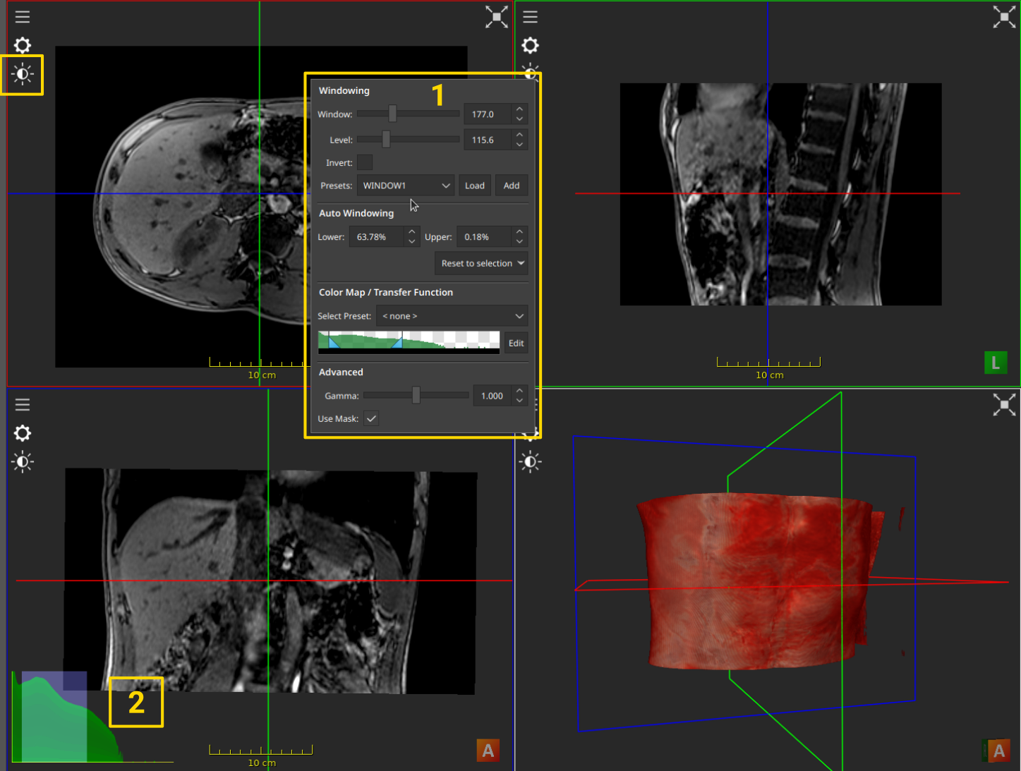
The Windowing Menu

A dedicated “Windowing” menu (1) is accessible by clicking the sun icon in the top left of a view. The exact value of the window and the level can be set there, and presets can be defined and restored later. The auto-windowing feature is used to reset the window and level value, so that the entire range of the image is visible.

For 3D images, separate windowing values are used for the slice views and the 3D view.

Windowing can also be controlled with mouse and keyboard by holding shift + holding left mouse-button + moving the cursor. The direction of the cursor movement determines the windowing change as such:

• up: increase the size of the window

• down: decrease the size of the window

• left: decrease the level

• right: increase the level

The currently applied windowing can also be displayed persistently by right-clicking a view, and selecting Show Histogram in the context menu. This will display an interactive histogram in the bottom-left corner of the view (2), where the blue rectangle represents the window. This can also be useful to better understand the keyboard and mouse interaction. Interacting with the blue rectangle is another way to control the windowing.

Blending

When two or more images of the same type are loaded and displayed in the 2D or MPR views, it can be useful to display them in a way that all are visible at the same time where they overlap. For example, this can be used to evaluate a registration, the effects of a filtering operation, or to move one of the two images so that they are aligned. This is referred to as “blending”.

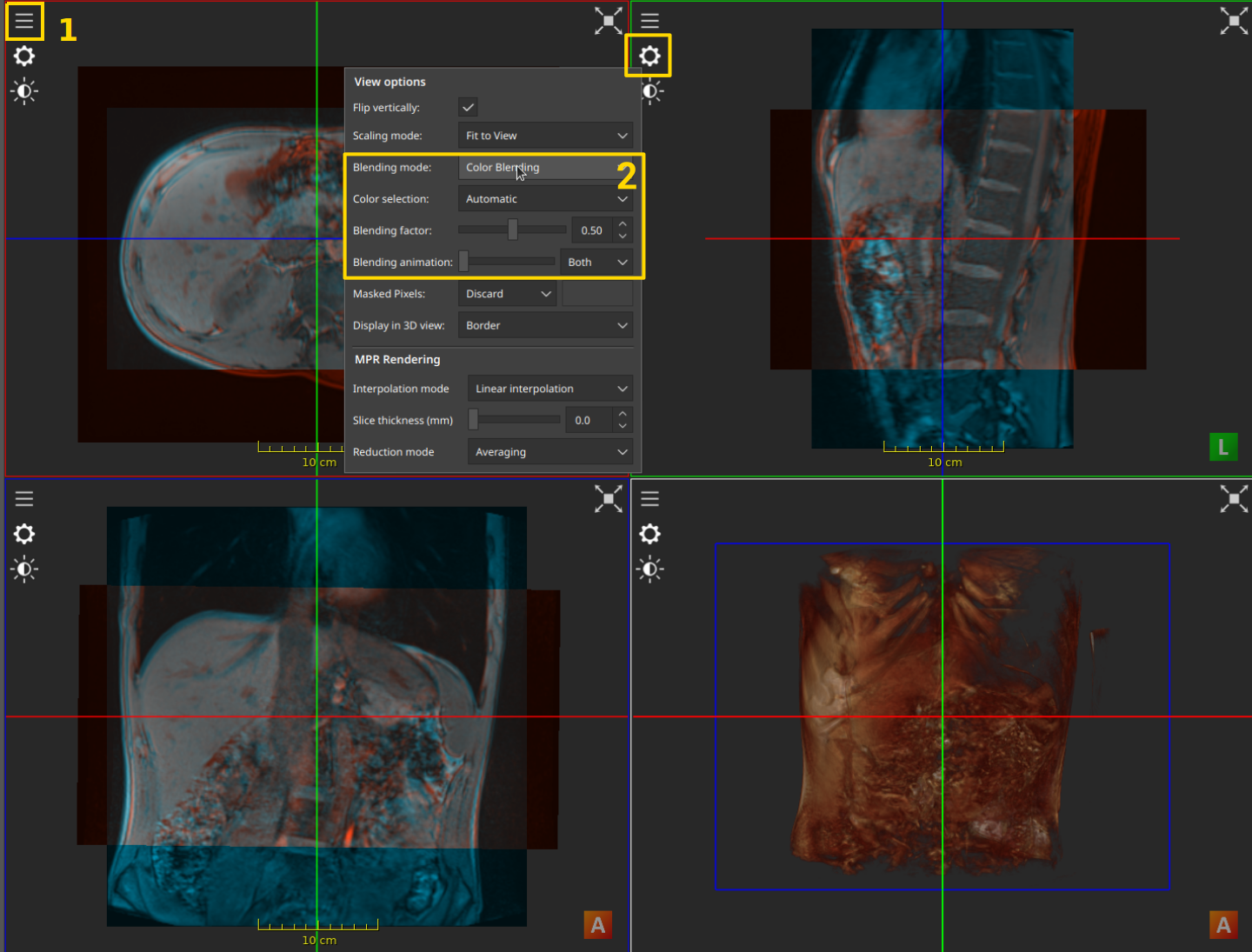
The blending options that are available under the View Options

After selecting the desired data with the Data Selection Button (1), the options to control blending are available in the “View Options” (the cog icon in the top left) menu (2). The main types of blending are:

• Alpha Blending: the images are shown with different levels of transparency. The blending factor controls how transparent the images are.

• Color Blending: the images are assigned a different color, and the combination of all colors is displayed. The blending factor controls the contribution of each image to the final color.

• Checkerboard Blending: only one of the images is shown in each square of the checkerboard. The view can be panned around so that the checkerboard is centered around a different area.

In alpha and color blending modes, the factor can be controlled with mouse and keyboard, by holding alt + holding left mouse button + moving the cursor left and right. Moving the cursor to the left will decrease the blending factor, moving it to the right will increase it.

Interaction list

The table below describes the possible interactions.

Button	Modifier Key	2D View	MPR View	3D View
Left		Zoom		Rotation
	Shift	Window/Level
	Control		Rotation
	Alt	Blending of multiple images
Middle		Change focus frame	Plane translation	Zoom
	Control	Rotation
Right		In-plane translation
Wheel		Change focus frame	Next/previous plane	Zoom
	Control	Change focus frame		Zoom

Visualizing Data in the ImFusion Suite

Warning

The following functionality is only available if the ImFusion Suite is installed and included in your system’s PATH.

A practical way to visualize one or multiple images is to start an ImFusion Suite instance from Python. This can be done via the open_in_suite() function:

>>> image_set_1 = imfusion.SharedImageSet()
>>> image_set_2 = imfusion.SharedImageSet()
>>> mesh = imfusion.Mesh()
>>> imfusion.open_in_suite([image_set_1, image_set_2, mesh])  

This is a (hopefully temporary) one-way solution only meant for visualization and not processing: changes in the Suite cannot be transferred back to the Python interpreter.

With this, you should have the basic knowledge to write your first scripts with the ImFusion framework. The following chapters will describe the introduced parts in more detail.