Annotation

The Annotation tab allows you to annotate the currently loaded dataset.
Different Annotation Actions can be selected via the Annotation Drop-Down Menu on the right of the tab.

Only one dataset can be loaded at a time, but browsing through the whole database can be easily done using the bottom table showing the thumbnail of all datasets. A single click on a thumbnail will unload the current dataset and load the selected one. Left and right arrow keys also allow to load the next (or previous) dataset in the list.
All annotations are saved automatically when the data is unloaded or the application is closed.
If you want to prompt the application to save the annotations (and the project file for local project) immediately, you can click on the icon  for local projects or
  for remote ones.
Other than by using the Undo functionality, it is not possible to revert a change in the annotation.
for remote ones.
Other than by using the Undo functionality, it is not possible to revert a change in the annotation.
Windowing presets can be defined using the display options of the views ( ).
When adding a new preset for the windowing values which are currently active, the preset can be either saved for the current dataset only, or saved for all the datasets with the same modality.
).
When adding a new preset for the windowing values which are currently active, the preset can be either saved for the current dataset only, or saved for all the datasets with the same modality.
Note
For a better user experience, we recommend using the keyboard shortcuts (see Keyboard Shortcuts).
Common tools
Pointer
The default interaction mode to visualize the data. Clicking on the views lets you modify them, but no annotation is performed. The layout of the views can be changed using the buttons.
A button “Consider annotated, even if empty” can be checked to mark the dataset as annotated. This can be used to indicate that a given dataset has been processed even it its annotation is empty, for example if it did not contain the structure of interest. Other features of ImFusion Labels which depend on whether a dataset is annotated (for example, filtering or exporting) will treat this dataset as if it had been annotated. For image sequences, this flag can be set on each image of the sequence. Images that have been marked as such can be seen in red (instead of the light-green for actually annotated images) on the scrollbar.
Define ROI
This tool lets you define a Region of Interest (ROI) within the loaded image/volume. The pixels outside of the region of interest will be hidden or displayed differently (depending on the settings). Defining a ROI lets you focus on the interesting part of the image, and makes other tools more efficient by limiting the amount of data they need to process. The ROI of each image is saved with the project.
Pixelwise Annotation
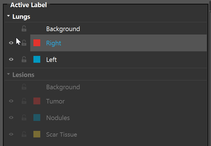
For segmentation projects, different modes of interaction/annotation are available in the right panel. The different labels of the project can be selected in the Active Label table. An additional label called “Background” is automatically added and is visualized as transparent.

Two icons are shown for each label: the eye icon indicates the visibility of the label value, while the lock indicates whether a label value can be overriden by the current annotation action. Click on the icon to toggle on/off the state of the labels. By default, all labels are visible and unlocked.
At any moment, the labels of a project can be modified in the Settings (the icon in the top-right): new labels can be added, and existing labels can be either modified or removed.
If the project has multiple layers (see Layers), the Active Label table will display all layers of the Project as a single table. The currently active layer and its labels are painted in full opacity, while other layers are painted in semi-transparent. The table allows selecting labels in the active layer and switching between layers.
Brush
Paint the active (i.e. currently selected) label into the image/volume. The brush takes into account the image intensities in order to reduce leaks and overpainting. Left-click paints the current label, while right-clicks erases it.
Note that the current contrast and brightness of the image views is taken into account by the adaptive brush.
Different options on the brush can be set from the Brush options panel:
Size Controls the size of the brush.
Adaptiveness Controls the adaptiveness of the brush, i.e. how much it adapts to the image. An adaptiveness of 0.0 means that the brush does not take into account the image at all, which means that the brush will always be a full sphere.
Image Noise Suppression Controls the suppression of the image noise as accounted by the adaptiveness of the brush. It is recommended for annotation of ultrasound images.
Smoothing Defines the smoothness of the image used for the adaptive brush. Setting this option on makes the labels smoother and less noisy.
Contiguous Defines whether all pixels labeled by the brush should be connected to the pixel of the mouse pointer.
2D Brush When painting, only label pixels of the current slice, and not those of its neighbours. Note that if the slice is oblique (i.e. not aligned with the voxels of the image) this might produce stairsteps artifacts. Only applicable to 3D datasets.
Link 2D Views When painting, scroll through other slices such that they are focused on the center of the brush. Only applicable to 3D datasets.
The different labels can be “locked” by pressing the lock icon. When a label is locked, it will not be erased if you try to draw a different label on top.
Furthermore, two buttons allow you to either clear the whole label map, or only the current label.
If you need to temporarily disable the “Brush” functionality (for example to modify the visualization of the data), you can press the space-bar key. This will also grey-out the side panel. Press space-bar again to reenable the action.
Erase
This tool is used to erase parts of the label map.
The “Eraser” is a subset of the Brush functionality, and is used to erase the labels around the cursor. Only unlocked labels are erased with this tool.
The “3D Scissors” can be used to manually cut out parts of the label map, by drawing directly in the views. Note that the scissors will not cut a label that has been locked.
The “Clear Label Map” buttons can be used to remove certain labels from the entire image. “Clear Active Label” will only remove the currently selected label type, whereas “Clear All Labels” will remove any label type that is not currently locked. If an image sequence is being labelled, a drop-down list can be used to chose in which frames the labels should be removed.
Interactive Segmentation
Propagate the current labels to the whole image (or the selected ROI). The user is expected to label partially at least one object of interests with some brush strokes, as well as the background.
The propagation starts when the button Run Segmentation is clicked, or automatically if the option is enabled. The algorithm then runs in the background and updates the progress bar in the Annotation panel. When the segmentation result is ready, it gets displayed in the views with a lower opacity than the original labels.
As soon as the user updates the strokes, the segmentation can be re-computed. When the result is satisfactory, the button Accept Result allows to set it as the current label map.
In this mode, a “locked” label will not be propagated and will be kept as is.
Note that the current contrast and brightness of the image views is taken into account by the algorithm.
Tip
The selected label-value (e.g. the background) in the Active Label list can be exported/imported: right-click on the selected value and choose the “Export/Import selected Labels” from the list of actions.
Slice Interpolation
This action is only available for 3D datasets. It interpolate the content of some slices to all the slices inbetween.
The action expects as input a label map with several 2D slices (in one or several of the three main directions) already labelled, for instance drawn by the Brush action with the 2D Brush option. The interpolation only considers the shape of the slice annotations, but not the image content.
Refine
Shows post-processing operations to be performed on the label map. The operations apply only on the active label selected in the table.
Keep largest component
Remove small components
Fill holes
Smooth label map either with a Gaussian filter or a median (more robust) filter
Erode/dilate label map
Run an image-based refinement in a narrow band around the current borders of the label
Connected Components
Split the current label map into components based on its connectivity.
By clicking on “Start”, a components analysis of the label map is started in the background. When it is finished, the label map is split into distinct components, each identified with a different pastel color. By hovering the cursor over a component in the views, it’s number is displayed. Alternatively, “Use Current Labels as Components” skips the component analysis and uses the existing labels as components. This can be useful to re-assign existing labels or splitting components manually.
Locked labels are not considered during the analysis and will remain in their current state. Their assignment cannot be changed. Which label is locked can only be configured before the component analysis.
If the splitting is too coarse (e.g. two components are merged because of a small interface), the components can be further split. The “Split Manually” tool can be used to draw a shape along which the components will be split. Everything within the shape becomes a new component. The “Split Along” tool will split the components along one of the current view axes. The view axes can be rotated with a right-click drag to cut along different angles. The components analysis can be started again from this current state, for example if the tools were used to split two parts of a component.
To assign labels, check the “Assign Manually” button and left-click on a component in one of the views. Select the desired label in the menu. The “Set Unassigned Components to” button can be used to assign a label to multiple components at once. The special “Previous Label” entry can be used to preserve the label that the component had at the beginning.
Once a label has been assigned to each of the components, the “Accept” button is enabled. When accepted, the components and their label assignment become the actual label map.
If “Auto-Start” is checked, the components analysis is started automatically whenever the current frame is changed, as well as when the splitting tool is used.
Draw Contour
Draw the contour of an object to be labeled using various kinds of annotations:
Closed Polyline Polygon defined by a series of straight line segments. Only for 2D datasets.
Closed Spline Contour defined by a series of 2D curves interpolated between the control points
Closed Loop Special annotation for round objects. The first three control points define an ellipse, then each segment can be refined by adding a furter control point in between.
Open Spline This annotation type is useful for very thin structures that can be well approximated by their centerline.
Note
The closed annotations are only available for 2D datasets.
Such contours are defined by a series of points. Left-click on the image to start drawing a contour with the selected label; new points are automatically added until you right-click for the final point. Once the annotation has been defined, you can adjust it by moving the control points (right-click on a point and drag it around) or the whole annotation (left-click on a pont and drag it around). It is also possible to add a new control point by left-clicking on an existing point while pressing Ctrl down.
For the closed annotations, the Auto-Refine parameter lets you automatically adjust the label map to match the content of the image. The Refinement Margin parameter controls the width of the area around the drawn contour that the refinement should run on.
For the open annotations, the Radius parameter defines the width around the drawn contour of the actual structure, while the Adaptiveness controls how much the written labels should adapt to the content of the image.
The interactivity with the spline in the views can be toggled on or off by pressing the Draw Contour button. When toggled off, the views can be navigated with the usual interactions.
After the annotation is defined, a preview can be seen in the views. The preview is updated whenever the annotation parameters or the spline itself are modified. Once the preview looks satisfactory, the Accept button will apply it to the label map. The current contour can always be removed with the Discard button
Frames that contain a contour are displayed in yellow on the scrollbar.
Deform
With this tool, the label map can be deformed locally by pushing and pulling it. To start the deformation, move the mouse while holding the mouse left button down. The deformation will be applied when you release the mouse button.
The locality of the deformation is indicated by the circle, and can be modified by using the “Size” slider.
Note that deformations over large distances can have unexpected effects. For best results, you should compose multiple deformations over small distances.
You can always undo deformations either with the Keyboard Shortcuts or using the Undo/Redo action.
Threshold
Set all pixels of the image within a given intensity range to the currently selected label.
Adjust the sliders to select the appropriate intensity range.
Label Propagation
Note
This mode is only available for multi-frames datasets, i.e. most of the time temporal sequences like video clips.
Propagate automatically the selected labels of the current frame to other frames. Multiple labels (or even all) can be selected to propagate them at the same time. Propagated frames are displayed in dark green on the scrollbar.
Three modes are available:
Label Map Interpolation Match the label map of the current frame to the next labeled frame and interpolate it linearly in-between.
If the mode is set to “Propagate over all subsequent frames”, it will be matched instead to the last labeled frame. This mode does not use the image information, but only the label maps.
Image-based Tracking Propagate the label map by registering successively frames of the dataset.
If the mode is set to “Propagate over all subsequent frames”, all successive frames will be matched to the current frame. If the mode is set to “Propagate and update reference with labeled frames”, the reference frame will not necessarily be the current frame, but will be updated every time a labeled frame is encountered.
Both Combine the two previous approaches: initialize with the interpolated deformation, then runs an image-based refinement between successive frames.
Both propagation modes are based on a modified multi-scale Demons registration algorithm, whose parameters can be tuned to control the regularization of the tracking.
If Propagate until the next labeled frame is selected, the propagation is interrupted as soon as a frame which already contains the propagated labels is reached.
Template Deformation
Note
This functionality is experimental and not shipped in production yet.
Use an already segmented image as a template to segment the current image: the template image will be registered to the new one, and the same deformation will be applied to the template label map. This mode is particularly useful for segmentation applications that require a strong shape prior.
1. Template Selection First select one of the templates from the list, and click on Load Template. Available templates are datasets from the project that are compatible with the current dataset and have already been segmented. Once loaded, both the template image and labels are available and can be visualized. By default and for the sake of simplicity, only the template label map is being shown but this can be customized using the check boxes.
2. Global Registration The loaded template can then be globally adjusted either manually or automatically:
Manual Alignment allows to move the template interactively. When this mode is toggled on, the user can hold right-click in the image views and move the mouse to apply a translation to the template. Click again on the button to disable this mode.
Show Transformation Editor opens a dialog with more parameters of the transformation. In particular, rotations, shearing and scalings can be applied to the template.
Run Global Registration starts an automatic registration algorithm which is going to align as much as possible the template image with the current dataset. The optimized transformation can be either rigid (only translation and rotation) or affine (with shearing and scaling).
3. Template Deformation allows to further adjust the template to the current dataset with a dense deformation field. When the button Run Deformable Registration is clicked, algorithm runs a multi-scale registration method that can be controlled with the different parameters. The Reset Deformation button removes the deformation but preserves the global alignment matrix of the template.
Finally, click on Accept Label Map to set the deformed template labels as the new label map for the current dataset.
Replace Values
Replace some indices of the label maps with other values.
Import
Import a label map from a file on the disk, from another layer in the same project or a mesh file on disk (only in 3D).
After loading a file, the segmentations from the file can be mapped to the current layer. By default, labels are mapped according to their (pixel) value. The result of the mapping is previewed in the views. The opacity of the existing segmentations is automatically reduced to 0, so that only their outline is visible. This makes it easier to compare the imported segmentations with the existing onces.
The existing segmentations are not cleared. This means if the default mapping of the background is removed, the existing segmentations are combined with the imported ones.
Locked labels will not get overwritten by the import.
To apply the imported segmentations to the layer, click “Import”.
When importing a mesh, it is assumed to be in the same coordinate system as the image (including origin and orientation) and should represent a closed surface. All pixels enclosed in the mesh will be set to one label, all the other ones will be set to background.
Run Script
Run either a Python algorithm or an ImFusion Workspace file, and set its result as the new label map.
Current labels can be locked so that they won’t be modified by the script.
Python Algorithms In order to learn how to write Python algorithms for ImFusion Labels, please go the page Writing Algorithms.
ImFusion Workspaces Those workspace files are the same as in the ImFusion Suite. The lastly created image will be selected as the new label map.
In order to reference the dataset as input of an algorithm, use the UID image. The current label map is available as the UID label. More details on how to write workspace files can be found in the ImFusion SDK documentation.
Undo / Redo
The undo tab shows a history of modifications done to the label map. The list shows a short description of the operation, as well as when it happened. When selecting any item in the list, the state of the label map at the time will be restored.
When selecting an earlier undo level, all the levels after are grayed out. Grayed out levels will be deleted when the next undo level is created, so be careful.
The undo history is not persisted, and will be discard when the dataset is changed.
You can configure the maximum memory usage of this feature in the settings. When the maximum is exceeded, the oldest undo data will be removed.
Geometric Annotations
The main interaction in geometric annotation projects is the Geometric Annotation action. It provides tools to create and modify different annotation types, like landmarks, bounding boxes or line measurements. All currently defined annotations on the active datasets are displayed in a list, grouped by their corresponding label.
An existing annotation can be focused by either selecting it in the list, or by clicking on it in the views. The currently focused annotation can be deleted by pressing the Del key. By checking the Center Views on Selected Annotation checkbox, the views will be automatically re-centered when selecting an annotation in the list.
If you need to temporarily disable the editing functionality while you are adding an annotation (for example to modify the visualization of the dataset), you can press the space-bar key. Press space-bar again to reactivate the editing functionality.
Landmarks
To add a new landmark, select a landmark type, and press the “Add landmark” button (or the keyboard shortcut A). Then, move the mouse over the desired position in the views and press the left mouse button. Landmarks can be added in the 3D View too: when a left-click is performed with the mouse the first hit-point on the data’s surface will be the position of the landmark.
After a landmark is set, it is possible to modify its position by left-clicking and dragging it in the views via the mouse (MPRs and 2D).
Line Measurements
To add a new line measurement, select a line measurement type, and press the “Add Line Measurement” button (or the keyboard shortcut A). Then, move the mouse over the desired position in the views, press the left mouse button to set the first point, move the mouse again to the next position and press left mouse button again to set the second point.
After a line measurement is set, it is possible to modify the positions of its end points by left-clicking and dragging them in the views via the mouse (MPRs and 2D). By left-clicking and dragging the line connecting the points, the complete line can be moved.
Bounding Boxes
To add a new bounding box, select a bounding box type, and press the “Add bounding box” button (or the keyboard shortcut A). Then, move the mouse over the desired position in the views and press the left mouse button to define a corner of the box. For 3D datasets, after two corners have been defined, move the cursor to a different slice view and click there to give the box the desired depth.
The currently focused bounding box can be resized by dragging its edges or corners, or moved by dragging its center. It can be deleted by pressing the Del key.